Advanced explanations

This guide is for users who want more control over how historical relationships are measured or used in a forecast explanation. Start with the customer-facing guides if your question is simply:

The examples below continue with the same retail df and future X_df from those guides.

Compare historical relationship analyses

explain() provides two complementary analyses:

Analysis	Useful when
Granger	You want a fast first pass focused on linear, lagged relationships
Transfer entropy	You expect nonlinear or more complex lagged relationships

Run both on the same data:

granger_signals = nixtla_client.explain(
    df=df,
    features=["price", "promotion", "temperature"],
    method="granger",
)

entropy_signals = nixtla_client.explain(
    df=df,
    features=["price", "promotion", "temperature"],
    method="transfer_entropy",
)

Feature	Granger	Transfer entropy
Price	0.000	0.502
Promotion	0.863	0.046
Temperature	0.137	0.452

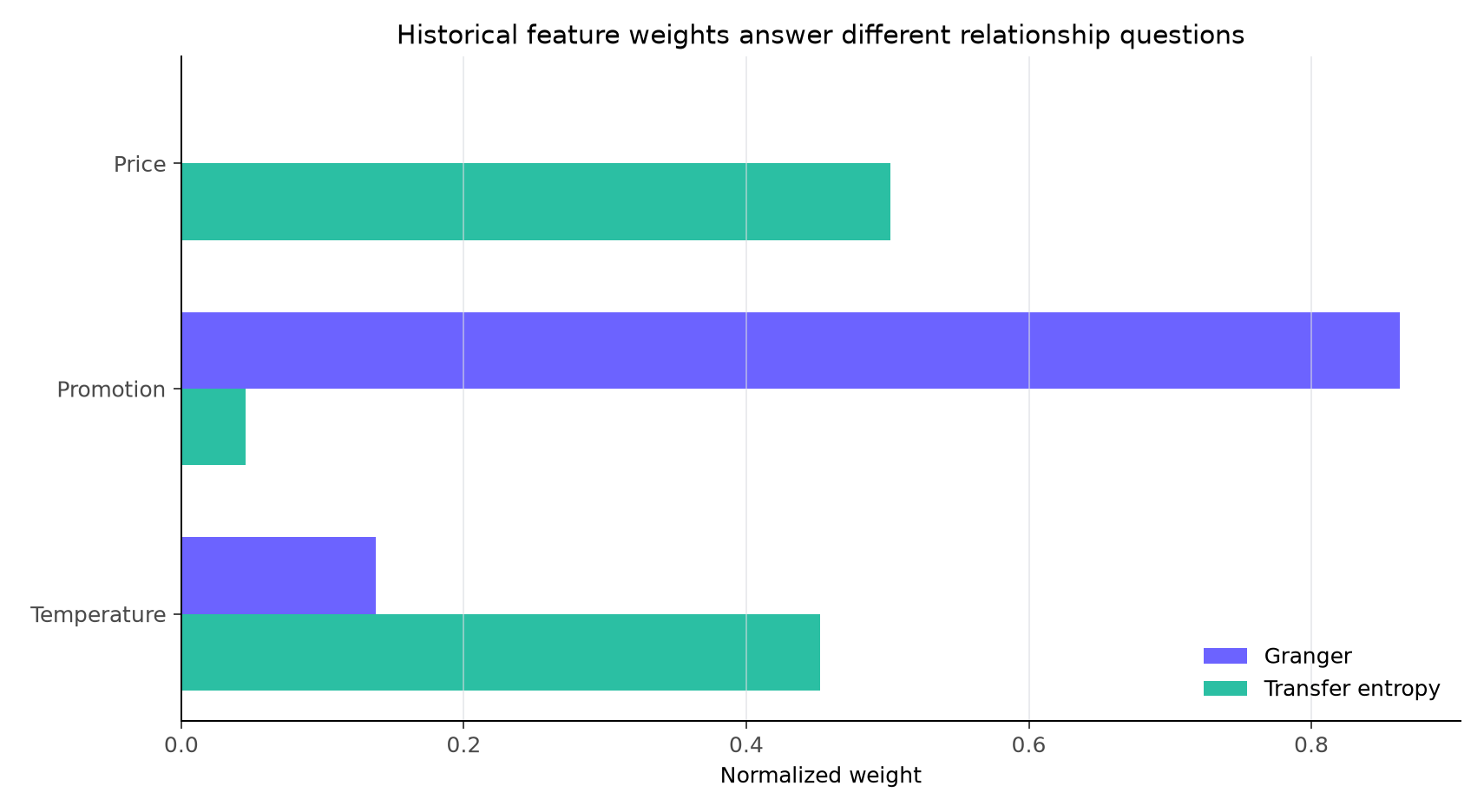
Grouped bars comparing Granger and transfer-entropy weights for price, promotion, and temperature — The analyses emphasize different patterns in the same historical data. Results were generated locally from TimeGPT 2.1.

The linear analysis emphasizes promotion. Transfer entropy finds more historical information in price and temperature. The useful question is not which analysis “wins,” but which relationship matches what you are investigating.

Allocate a forecast using historical relationships

TimeGPT can also use those historical weights to divide the movement of a forecast around its starting value:

"granger" and "transfer_entropy" appear in two different places. As the method argument to explain() (above) they screen historical relationships without a forecast. As feature_contributions_type in forecast() (below) they use those same relationship measures to allocate a forecast. Same names, two mechanisms.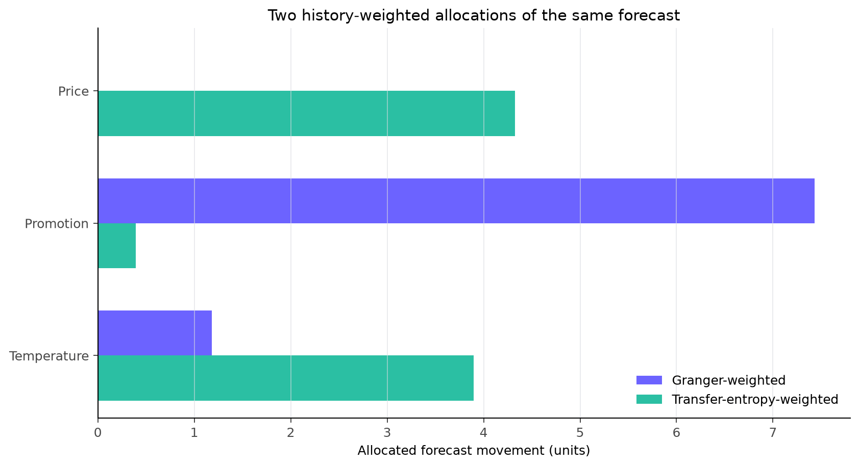

forecast = nixtla_client.forecast(
    df=df,
    X_df=X_df,
    h=14,
    freq="D",
    model="timegpt-2.1",
    feature_contributions=True,
    feature_contributions_type="granger",
)
granger_contributions = nixtla_client.feature_contributions.copy()

forecast = nixtla_client.forecast(
    df=df,
    X_df=X_df,
    h=14,
    freq="D",
    model="timegpt-2.1",
    feature_contributions=True,
    feature_contributions_type="transfer_entropy",
)
entropy_contributions = nixtla_client.feature_contributions.copy()

For the first promotion day, both views explain the same 92.01-unit forecast:

Input	Granger-weighted	Transfer-entropy-weighted
Price	0.00	4.33
Promotion	7.43	0.39
Temperature	1.18	3.90

Grouped bars showing two history-weighted allocations of the same retail forecast — Both allocations add to the same forecast movement, but distribute it using different historical evidence.

Use these views when you specifically want a forecast allocation grounded in a selected historical relationship analysis. Use SHAP when you want the standard prediction-level explanation.

Check whether a ranking is stable

A feature ranking can change when the historical window changes. Re-running the analysis over adjacent windows helps reveal persistent and temporary signals: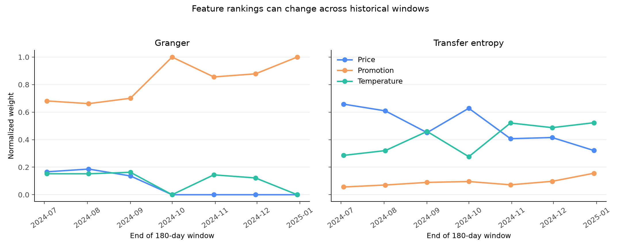

window_results = []

for end in range(185, len(df) + 1, 30):
    window = df.iloc[end - 180 : end]

    for analysis in ["granger", "transfer_entropy"]:
        result = nixtla_client.explain(
            window,
            features=["price", "promotion", "temperature"],
            method=analysis,
        ).assign(
            analysis=analysis,
            window_end=window["ds"].max(),
        )
        window_results.append(result)

weight_history = pd.concat(window_results, ignore_index=True)

Two line charts showing historical feature weights across rolling windows — Rolling 180-day windows show which historical signals persist and which depend on the selected period.

Stable rankings are easier to use operationally. A changing ranking is useful information too: it can point to seasonality, a business shift, or a data issue worth investigating.

Practical details

Output and additivity

Historical explain() weights are nonnegative and add to one. Granger-weighted and transfer-entropy-weighted forecast contributions add to TimeGPT together with base_value. Intervention contributions are calculated one input at a time and need not add up to the forecast.

Categorical inputs

List categorical columns in categorical_exog_list. Historical relationship analyses encode categories consistently before measuring lagged relationships. Treat the result as a ranking rather than a numeric distance between category labels.For any feature_contributions_type other than "shapley", categorical features cannot be combined with hist_exog_list when the request also covers historical timestamps, that is forecast(..., add_history=True). The historical/future column mapping cannot be represented faithfully once the categorical columns are split out, so the request is rejected rather than returning a silently wrong explanation. Either keep the exogenous features all-numeric, drop hist_exog_list, or use "shapley". A plain forecast() call is unaffected and supports this combination.

Request limits

A request supports up to 75 explained features and 1,000,000 historical feature-observations. Transfer entropy generally takes more computation than Granger analysis.

When no signal is detected

If an analysis cannot distinguish the selected features, explain() returns equal weights. This can happen with short series, constant values, or a historical window that contains little predictive information.

Advanced explanations are most useful when the analysis question is explicit. Record the selected analysis and historical window alongside any result you share.

INTRODUCTION

SETUP

DATA REQUIREMENTS

FORECASTING

ANOMALY DETECTION

USE CASES

REFERENCE

About

Compare historical relationship analyses

Allocate a forecast using historical relationships

Check whether a ranking is stable

Practical details

​Compare historical relationship analyses

​Allocate a forecast using historical relationships

​Check whether a ranking is stable

​Practical details

Compare historical relationship analyses

Allocate a forecast using historical relationships

Check whether a ranking is stable

Practical details