What-If Forecasting: Price Effects in Retail

Introduction

Pricing decisions significantly impact retail demand. TimeGPT makes it possible to forecast product demand while incorporating price as a key factor, enabling retailers to explore how the forecast changes under different pricing assumptions. This tutorial demonstrates how to use TimeGPT for scenario analysis by forecasting demand under various pricing conditions. You’ll learn to incorporate price data into forecasts and compare forecasts across different price assumptions.

A scenario forecast is not a price-effect estimate. Changing a future price and re-forecasting shows the model’s conditional forecast given that price: a relationship learned from how price and demand moved together historically. In retail history, prices are rarely changed at random: markdowns respond to slow sales, and promotions are timed to seasons. The learned relationship therefore mixes the true effect of price with the pricing policy that set it, so the difference between two scenario forecasts can overstate or understate the real demand response to a price change. This is most pronounced for price moves outside the historically observed range.Use these scenarios to explore and stress-test assumptions, not to read off price elasticities. Before committing a pricing decision, validate the implied demand response with a price experiment or a holdout test.

What You’ll Learn

How to forecast retail demand using price as an exogenous variable
How to run what-if scenarios with different pricing strategies
How to compare baseline, increased, and decreased price forecasts
How to interpret scenario forecasts and why they are not price-elasticity estimates

How to Forecast Sales with Pricing Scenarios

Step 1: Import required packages

Import the packages needed for this tutorial and initialize your Nixtla client:

import pandas as pd
import os

from nixtla import NixtlaClient

Initialize the Nixtla client:

nixtla_client = NixtlaClient(
    api_key='my_api_key_provided_by_nixtla'
)

Step 2: Load the M5 dataset

Let’s see an example on predicting sales of products of the M5 dataset. The M5 dataset contains daily product demand (sales) for 10 retail stores in the US. First, we load the data using datasetsforecast. This returns:

Y_df, containing the sales (y column), for each unique product (unique_id column) at every timestamp (ds column).
X_df, containing additional relevant information for each unique product (unique_id column) at every timestamp (ds column).

from datasetsforecast.m5 import M5

Y_df, X_df, S_df = M5.load(directory=os.getcwd())
Y_df.head(10)

unique_id	ds	y
FOODS_1_001_CA_1	2011-01-29	3.0
FOODS_1_001_CA_1	2011-01-30	0.0
FOODS_1_001_CA_1	2011-01-31	0.0
FOODS_1_001_CA_1	2011-02-01	1.0
FOODS_1_001_CA_1	2011-02-02	4.0
FOODS_1_001_CA_1	2011-02-03	2.0
FOODS_1_001_CA_1	2011-02-04	0.0
FOODS_1_001_CA_1	2011-02-05	2.0
FOODS_1_001_CA_1	2011-02-06	0.0
FOODS_1_001_CA_1	2011-02-07	0.0

For this example, we will only keep the additional relevant information from the column sell_price. This column shows the selling price of the product, and we expect demand to fluctuate given a different selling price.

X_df = X_df[['unique_id', 'ds', 'sell_price']]
X_df.head(10)

unique_id	ds	sell_price
FOODS_1_001_CA_1	2011-01-29	2.0
FOODS_1_001_CA_1	2011-01-30	2.0
FOODS_1_001_CA_1	2011-01-31	2.0
FOODS_1_001_CA_1	2011-02-01	2.0
FOODS_1_001_CA_1	2011-02-02	2.0
FOODS_1_001_CA_1	2011-02-03	2.0
FOODS_1_001_CA_1	2011-02-04	2.0
FOODS_1_001_CA_1	2011-02-05	2.0
FOODS_1_001_CA_1	2011-02-06	2.0
FOODS_1_001_CA_1	2011-02-07	2.0

Step 3: Forecast demand using price as an exogenous variable

In this example, we forecast for a single product (FOODS_1_129_) across all 10 stores. This product exhibits frequent price changes, making it ideal for modeling price effects on demand. Learn more about using exogenous variables in TimeGPT.

products = [
    'FOODS_1_129_CA_1', 'FOODS_1_129_CA_2', 'FOODS_1_129_CA_3', 'FOODS_1_129_CA_4',
    'FOODS_1_129_TX_1', 'FOODS_1_129_TX_2', 'FOODS_1_129_TX_3',
    'FOODS_1_129_WI_1', 'FOODS_1_129_WI_2', 'FOODS_1_129_WI_3'
]

Y_df_product = Y_df.query('unique_id in @products')
X_df_product = X_df.query('unique_id in @products')

Merge the sales (y) and price (sell_price) data into one DataFrame:

df = Y_df_product.merge(X_df_product)
df.head(10)

unique_id	ds	y	sell_price
FOODS_1_129_CA_1	2011-02-01	1.0	6.22
FOODS_1_129_CA_1	2011-02-02	0.0	6.22
FOODS_1_129_CA_1	2011-02-03	0.0	6.22
FOODS_1_129_CA_1	2011-02-04	0.0	6.22
FOODS_1_129_CA_1	2011-02-05	1.0	6.22
FOODS_1_129_CA_1	2011-02-06	0.0	6.22
FOODS_1_129_CA_1	2011-02-07	0.0	6.22
FOODS_1_129_CA_1	2011-02-08	0.0	6.22
FOODS_1_129_CA_1	2011-02-09	0.0	6.22
FOODS_1_129_CA_1	2011-02-10	3.0	6.22

Let’s investigate how the demand, our target y, of these products has evolved in the last year of data.

nixtla_client.plot(df, unique_ids=products, max_insample_length=365)

Historical retail demand showing intermittent sales patterns across 10 stores for FOODS_1_129 product — Historical retail demand showing intermittent sales patterns across 10 stores

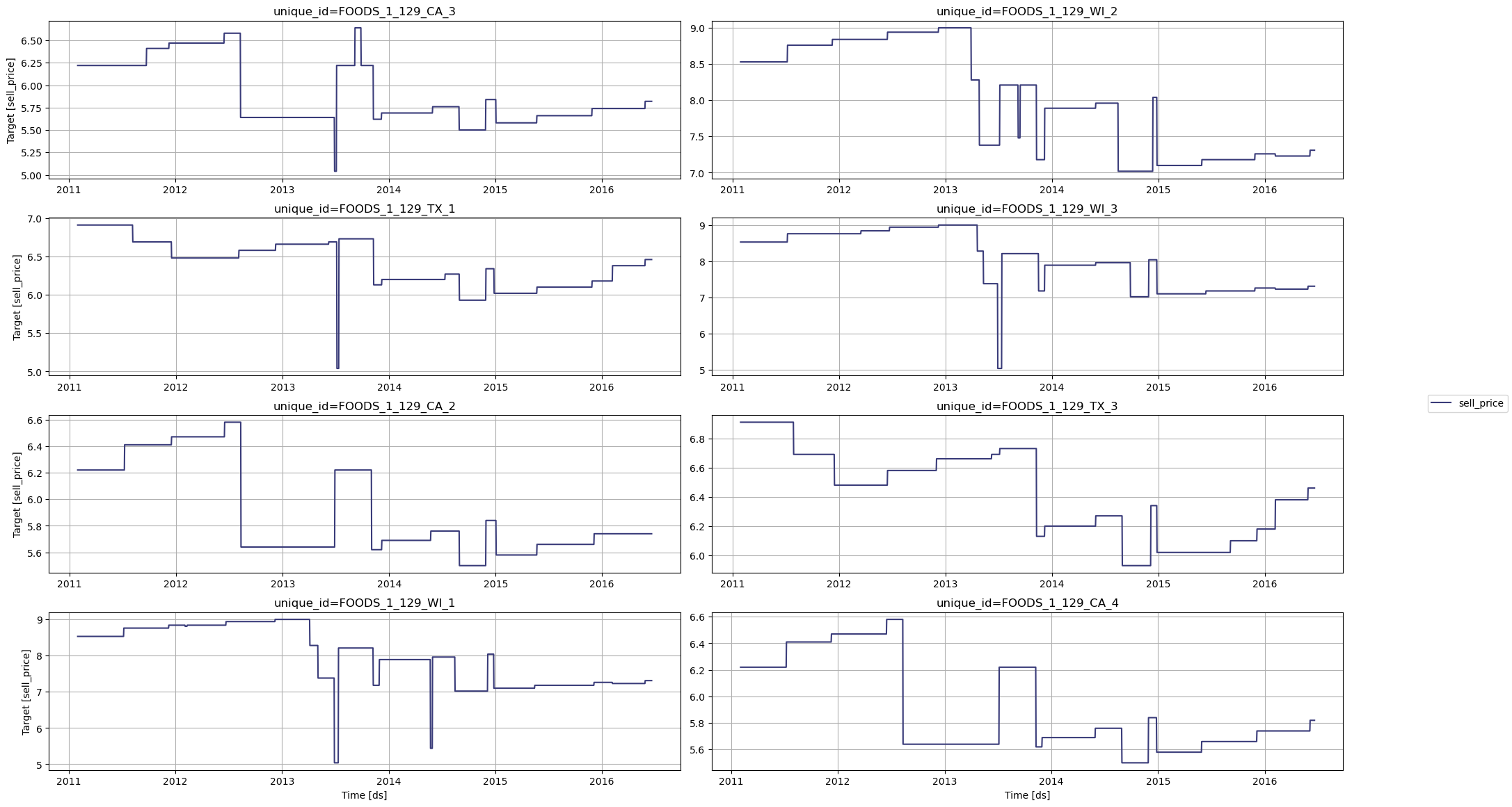
We see that in the California stores (with a CA_ suffix), the product has sold intermittently, whereas in the other regions (TX and WY) sales where less intermittent. Note that the plot only shows 8 (out of 10) stores. Next, we look at the sell_price of these products across the entire data available.

nixtla_client.plot(df, unique_ids=products, target_col='sell_price')

Historical pricing trends showing approximately 20 price changes from 2011 to 2016 for retail products — Historical pricing trends showing price changes over 5 years for retail products

We find that there have been relatively few price changes (about 20 in total) over the period 2011 to 2016. Let’s turn to our forecasting task. We will forecast the last 28 days in the dataset. To use the sell_price exogenous variable in TimeGPT, we have to add it as future values. Therefore, we create a future values dataframe, that contains the unique_id, the timestamp ds, and sell_price.

future_ex_vars_df = df.drop(columns = ['y'])
future_ex_vars_df = future_ex_vars_df.query("ds >= '2016-05-23'")

future_ex_vars_df.head(10)

unique_id	ds	sell_price
FOODS_1_129_CA_1	2016-05-23	5.74
FOODS_1_129_CA_1	2016-05-24	5.74
FOODS_1_129_CA_1	2016-05-25	5.74
FOODS_1_129_CA_1	2016-05-26	5.74
FOODS_1_129_CA_1	2016-05-27	5.74
FOODS_1_129_CA_1	2016-05-28	5.74
FOODS_1_129_CA_1	2016-05-29	5.74
FOODS_1_129_CA_1	2016-05-30	5.74
FOODS_1_129_CA_1	2016-05-31	5.74
FOODS_1_129_CA_1	2016-06-01	5.74

Next, we limit our input dataframe to all but the 28 forecast days:

df_train = df.query("ds < '2016-05-23'")

df_train.tail(10)

unique_id	ds	y	sell_price
FOODS_1_129_WI_3	2016-05-13	3.0	7.23
FOODS_1_129_WI_3	2016-05-14	1.0	7.23
FOODS_1_129_WI_3	2016-05-15	2.0	7.23
FOODS_1_129_WI_3	2016-05-16	3.0	7.23
FOODS_1_129_WI_3	2016-05-17	1.0	7.23
FOODS_1_129_WI_3	2016-05-18	2.0	7.23
FOODS_1_129_WI_3	2016-05-19	3.0	7.23
FOODS_1_129_WI_3	2016-05-20	1.0	7.23
FOODS_1_129_WI_3	2016-05-21	0.0	7.23
FOODS_1_129_WI_3	2016-05-22	0.0	7.23

Now, we can generate forecasts using TimeGPT (28 days ahead):

timegpt_fcst_df = nixtla_client.forecast(
    df=df_train,
    X_df=future_ex_vars_df,
    h=28
)
timegpt_fcst_df.head()

unique_id	ds	TimeGPT
FOODS_1_129_CA_1	2016-05-23	0.875594
FOODS_1_129_CA_1	2016-05-24	0.777731
FOODS_1_129_CA_1	2016-05-25	0.786871
FOODS_1_129_CA_1	2016-05-26	0.828223
FOODS_1_129_CA_1	2016-05-27	0.791228

We plot the forecast, the actuals and the last 28 days before the forecast period:

nixtla_client.plot(
    df[['unique_id', 'ds', 'y']],
    timegpt_fcst_df,
    max_insample_length=56
)

TimeGPT baseline forecast showing actual demand and 28-day ahead predictions for retail products — TimeGPT baseline forecast with 28-day ahead predictions for retail demand

Step 4: What-If Scenario Forecasting with Price Changes

What happens when we change the price of the products in our forecast period? Let’s see how our forecast changes when we increase and decrease the sell_price by 5%.

price_change = 0.05

future_ex_vars_df_plus = future_ex_vars_df.copy()
future_ex_vars_df_plus["sell_price"] *= (1 + price_change)

future_ex_vars_df_minus = future_ex_vars_df.copy()
future_ex_vars_df_minus["sell_price"] *= (1 - price_change)

Let’s create a new set of forecasts with TimeGPT.

timegpt_fcst_df_plus = nixtla_client.forecast(df_train, future_ex_vars_df_plus, h=28)
timegpt_fcst_df_minus = nixtla_client.forecast(df_train, future_ex_vars_df_minus, h=28)

Rename and combine the scenario forecasts:

timegpt_fcst_df_plus = timegpt_fcst_df_plus.rename(columns={'TimeGPT':f'TimeGPT-sell_price_plus_{price_change * 100:.0f}%'})
timegpt_fcst_df_minus = timegpt_fcst_df_minus.rename(columns={'TimeGPT':f'TimeGPT-sell_price_minus_{price_change * 100:.0f}%'})

timegpt_fcst_df = pd.concat([timegpt_fcst_df, 
                             timegpt_fcst_df_plus[f'TimeGPT-sell_price_plus_{price_change * 100:.0f}%'], 
                             timegpt_fcst_df_minus[f'TimeGPT-sell_price_minus_{price_change * 100:.0f}%']], axis=1)

timegpt_fcst_df.head(10)

unique_id	ds	TimeGPT	TimeGPT-sell_price_plus_5%	TimeGPT-sell_price_minus_5%
FOODS_1_129_CA_1	2016-05-23	0.875594	0.847006	1.370029
FOODS_1_129_CA_1	2016-05-24	0.777731	0.749142	1.272166
FOODS_1_129_CA_1	2016-05-25	0.786871	0.758283	1.281306
FOODS_1_129_CA_1	2016-05-26	0.828223	0.799635	1.322658
FOODS_1_129_CA_1	2016-05-27	0.791228	0.762640	1.285663
FOODS_1_129_CA_1	2016-05-28	0.819133	0.790545	1.313568
FOODS_1_129_CA_1	2016-05-29	0.839992	0.811404	1.334427
FOODS_1_129_CA_1	2016-05-30	0.843070	0.814481	1.337505
FOODS_1_129_CA_1	2016-05-31	0.833089	0.804500	1.327524
FOODS_1_129_CA_1	2016-06-01	0.855032	0.826443	1.349467

In this run, forecast demand increases when we reduce the price and decreases when we increase it: the direction most retailers would expect. Keep in mind that this reflects the association the model learned from this product’s pricing history; as cautioned above, the size of the gap between the scenarios, and for some products even its direction, should not be read as the causal effect of the price change. Finally, let’s plot the forecasts for our different pricing scenarios, showing how TimeGPT forecasts a different demand when the price of a set of products is changed.

nixtla_client.plot(
    df[['unique_id', 'ds', 'y']],
    timegpt_fcst_df,
    max_insample_length=56
)

What-if scenario comparison: baseline, +5% price increase, and -5% price decrease demand forecasts — What-if scenario comparison showing demand forecasts under different pricing strategies

In the graphs we can see that for specific products for certain periods the discount increases expected demand, while during other periods and for other products, price change has a smaller effect on total demand.

Conclusion

What-if forecasting with TimeGPT supports pricing discussions by:

Exploring how the demand forecast changes under different price assumptions
Comparing multiple pricing scenarios simultaneously
Incorporating exogenous variables for realistic predictions

Scenario forecasts are a starting point for a pricing conversation, not a substitute for measuring price effects: the differences between scenarios reflect learned associations, and their magnitude and direction can differ from the true demand response. Validate promising scenarios with price experiments or holdout tests before acting on them.

Next Steps

Explore intermittent demand forecasting with TimeGPT
Learn about fine-tuning models for better accuracy
Understand cross-validation for model evaluation
Scale forecasts with distributed computing

Important Considerations

This method assumes that historical demand and price behaviour is predictive of future demand, and omits other factors affecting demand. To include these other factors, use additional exogenous variables that provide the model with more context about the factors influencing demand.
Because historical prices were typically set in response to demand rather than at random, the measured relationship between price and demand is an association, not a causal effect. Treat scenario differences as directional input for planning, and rely on experiments or basket-level analysis when you need to know why demand changed.
This method is sensitive to unmodelled events that affect the demand, such as sudden market shifts. To include those, use additional exogenous variables indicating such sudden shifts if they have been observed in the past too.

INTRODUCTION

SETUP

DATA REQUIREMENTS

FORECASTING

ANOMALY DETECTION

USE CASES

REFERENCE

About

Introduction

What You’ll Learn

How to Forecast Sales with Pricing Scenarios

Step 1: Import required packages

Step 2: Load the M5 dataset

Step 3: Forecast demand using price as an exogenous variable

Step 4: What-If Scenario Forecasting with Price Changes

Conclusion

Next Steps

Important Considerations

​Introduction

​What You’ll Learn

​How to Forecast Sales with Pricing Scenarios

​Step 1: Import required packages

​Step 2: Load the M5 dataset

​Step 3: Forecast demand using price as an exogenous variable

​Step 4: What-If Scenario Forecasting with Price Changes

​Conclusion

​Next Steps

​Important Considerations

Introduction

What You’ll Learn

How to Forecast Sales with Pricing Scenarios

Step 1: Import required packages

Step 2: Load the M5 dataset

Step 3: Forecast demand using price as an exogenous variable

Step 4: What-If Scenario Forecasting with Price Changes

Conclusion

Next Steps

Important Considerations