> ## Documentation Index
> Fetch the complete documentation index at: https://nixtla-enterprise-feat-simulate-and-explain.mintlify.site/llms.txt
> Use this file to discover all available pages before exploring further.
# Explain a forecast with SHAP
> See how each input moves an individual TimeGPT forecast up or down.
Use SHAP when someone asks:
> Why did TimeGPT produce this forecast?
SHAP starts from a reference forecast and shows how much each input moves the
prediction up or down.
```text theme={null}
starting value + input contributions = TimeGPT forecast
```
The values use the same unit as your target. If you forecast product demand, a
contribution of `+2` means two additional units in the model's forecast.
## Retail-demand example
A store uses its price, promotion plan, and temperature forecast to predict
demand for the next 14 days.
```python theme={null}
import numpy as np
import pandas as pd
from nixtla import NixtlaClient
nixtla_client = NixtlaClient(
# Defaults to os.environ["NIXTLA_API_KEY"]
api_key="my_api_key_provided_by_nixtla"
)
rng = np.random.default_rng(7)
n = 365
h = 14
t = np.arange(n + h)
price = 20 + 1.8 * np.sin(2 * np.pi * t / 90) + rng.normal(0, 0.35, n + h)
promotion = ((t % 42) >= 35).astype(int)
temperature = (
18
+ 9 * np.sin(2 * np.pi * (t - 30) / 365)
+ rng.normal(0, 0.8, n + h)
)
weekly = 6 * np.sin(2 * np.pi * t / 7)
demand = (
118
- 2.4 * price[:n]
+ 16 * promotion[:n]
+ 0.55 * temperature[:n]
+ weekly[:n]
+ rng.normal(0, 2.0, n)
)
dates = pd.date_range("2024-01-01", periods=n + h, freq="D")
df = pd.DataFrame(
{
"unique_id": "store-a",
"ds": dates[:n],
"y": demand,
"price": price[:n],
"promotion": promotion[:n],
"temperature": temperature[:n],
}
)
X_df = pd.DataFrame(
{
"unique_id": "store-a",
"ds": dates[n:],
"price": price[n:],
"promotion": promotion[n:],
"temperature": temperature[n:],
}
)
```
## Make and explain the forecast
Turn on `feature_contributions` when you call `forecast()`:
```python theme={null}
forecast = nixtla_client.forecast(
df=df,
X_df=X_df,
h=h,
freq="D",
model="timegpt-2.1",
feature_contributions=True,
)
contributions = nixtla_client.feature_contributions
```
The forecast for the first promotion day is:
```python theme={null}
promotion_day = X_df.loc[X_df["promotion"].eq(1), "ds"].min()
contributions.query("ds == @promotion_day")
```
| unique\_id | ds | TimeGPT | price | promotion | temperature | base\_value |
| ---------- | ---------- | ------: | ----: | --------: | ----------: | ----------: |
| store-a | 2025-01-06 | 92.01 | +0.21 | +0.55 | -0.59 | 91.85 |
The frame always has the ID and time columns, `TimeGPT`, one column per
feature in the order they were sent, and `base_value` last.
## Read the result
For January 6:
* The explanation starts at **91.85 units**.
* Price adds **0.21 units**.
* The planned promotion adds **0.55 units**.
* Temperature subtracts **0.59 units**.
* Together, they produce the **92.01-unit forecast** after rounding.
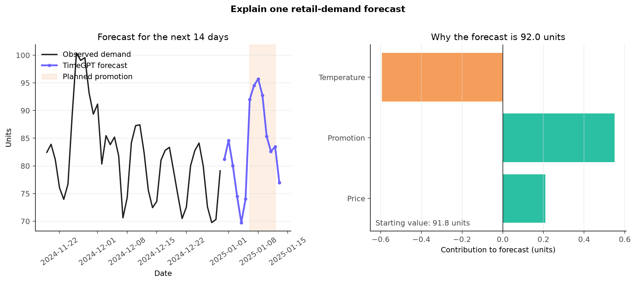 A positive contribution pushes the forecast above its starting value. A
negative contribution pushes it below. Neither sign is inherently good or bad;
it simply describes the direction of the model prediction.
## Find the biggest contributors
To summarize the entire forecast horizon, calculate the average absolute
contribution:
```python theme={null}
features = ["price", "promotion", "temperature"]
average_impact = (
contributions[features]
.abs()
.mean()
.sort_values(ascending=False)
)
average_impact
```
Use the row-level values when investigating a particular day. Use the average
when you need a quick view across the complete forecast.
SHAP explains how TimeGPT combined the available inputs for this forecast. Use
it to investigate surprising predictions, communicate forecasts, and decide
where to look next.
## Next
* [Test forecast sensitivity](/forecasting/explanation/intervention)
* [Find predictive signals in
history](/forecasting/exogenous-variables/causal-explanations)
* [Advanced explanations](/forecasting/explanation/advanced-explanations)
A positive contribution pushes the forecast above its starting value. A
negative contribution pushes it below. Neither sign is inherently good or bad;
it simply describes the direction of the model prediction.
## Find the biggest contributors
To summarize the entire forecast horizon, calculate the average absolute
contribution:
```python theme={null}
features = ["price", "promotion", "temperature"]
average_impact = (
contributions[features]
.abs()
.mean()
.sort_values(ascending=False)
)
average_impact
```
Use the row-level values when investigating a particular day. Use the average
when you need a quick view across the complete forecast.
SHAP explains how TimeGPT combined the available inputs for this forecast. Use
it to investigate surprising predictions, communicate forecasts, and decide
where to look next.
## Next
* [Test forecast sensitivity](/forecasting/explanation/intervention)
* [Find predictive signals in
history](/forecasting/exogenous-variables/causal-explanations)
* [Advanced explanations](/forecasting/explanation/advanced-explanations)